

Motivation
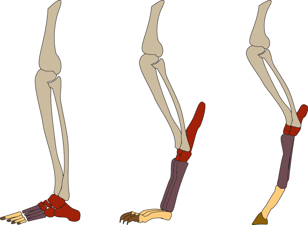
When we look at the bio-mechanical differences between quadrupeds and bipeds, there are quite a plethora of striking differences that can be drawn. In general, quadrupeds, like cats and dogs, walk/run on their toes, known as digitigrade legs. In contrast bipeds, like humans, walk/run on both the balls of their feet as well as their heels, known as plantigrade legs. However, there are other striking examples within nature that break these conventions, like that of birds, who are classified as bipeds with digitigrade legs and rodents, who are quadrupeds with plantigrade legs.
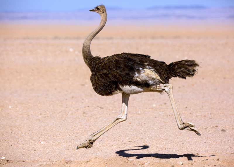
Biological studies have found that in general, digitigrade legs offer the user high gait velocities, while sacrificing stability/balance, while plantigrade legs offer the opposite. We can see the application of this by looking at two types of bipeds. Ostriches, whom bear digitigrade legs, can run upwards of 47 mph, while conversely, humans, with plantigrade legs, can only run upwards of approximately 18 mph.


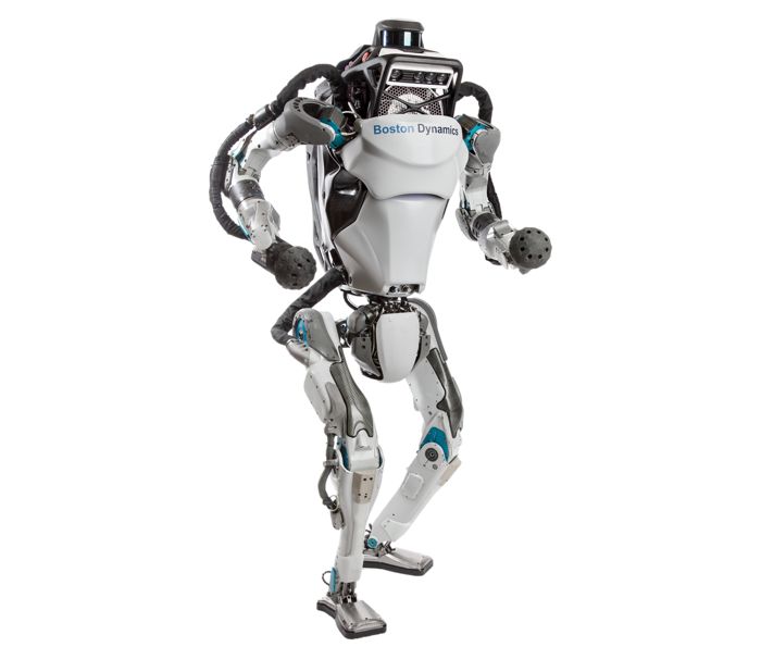
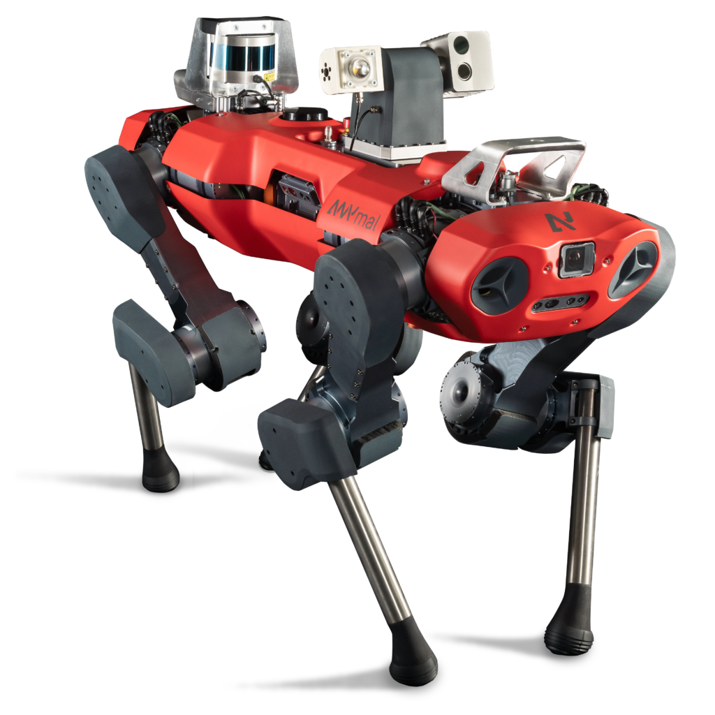
In the current design of legged robots, there is a tendency to develop feet that mimic very closely their biological counterparts, in that quadrupedal robots contain single-point contact at the feet (digitigrade, like that of the Anybotics Anymal) while bipedal robots contain feet with a distributed point contact (plantigrade, like that of the Boston Dynamics Atlas). There are occasional examples in nature (and very often in works of fiction) where bipeds contain digitigrade legs and quadrupeds contain plantigrade legs. The generally accepted reasoning for choosing to design legged robots in this way is because quadrupeds are stable dynamic systems, and can afford the loss in stability with digitigrade legs, while bipeds are inherently unstable dynamic systems and need the additional stability earned from plantigrade legs to keep upright. The overlying question presented here is why are digitigrade legs better for outputting higher gait velocities while plantigrade legs are less effective at achieving higher gait velocities and determine if there is an optimal design configuration in leg/foot geometry/control for some of the most common applications in legged robotics.
In this project, we investigate the coupling of gait velocity with both digitigrade and plantigrade legs. With this study, we can offer better insight into design decisions for legged robot design by fully understanding the performance achieved by these types of legs. In short, does the incorporation of ankle joints improve the gait velocity of legged robots?
We postulate the following:
· Digitigrade locomotion provides for faster gait velocity
· The incorporation of a third actuated “foot” linkage will reduce gait velocity
· By applying more torque within the ankle joint during the contact stage of the gait, higher gait velocities for plantigrade locomotion will be achieved
· With a high enough ankle joint torque, we will effectively have a digitigrade leg, however as ankle joint torque continues to increase, there will be an optimal setting for maximum gait velocity
Experimental Proposition
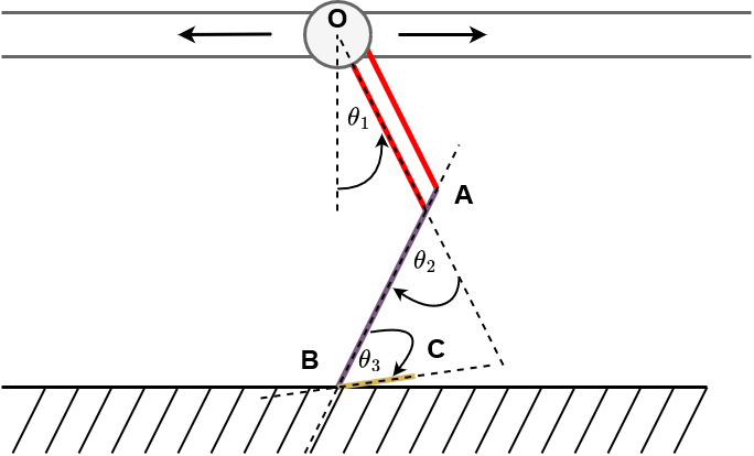
To investigate these hypotheses, we can first look at two simplified models for both digitigrade and plantigrade locomotion. For digitigrade locomotion, we can model the system with 2-DoF where the impact with the ground is a single point contact. Conversely, for plantigrade locomotion, we can model the system with 3-DoF where the ground impact is distributed across a single link acting as the foot. We can model the three joint angles as shown below in Figure 4. With the ankle joint set to pi rad and angular velocity set to 0 rad/s; we can assume the leg to be in a digitigrade configuration.
For this design, we placed the hip and knee motors necessary to actuate this leg at the base of the leg (joint O) while placing the motor for the ankle actuation at the knee joint (joint A). The hip joint will be actuated by direct drive, whereas the knee joint will be actuated via a parallel linkage and the ankle joint had a series of rubber bands placed in a manner to simulate effective ankle impedance. The base of the leg is fixated to a linear rail with a fulcrum assembly to enable 2-DoF along the transverse and vertical axes. To carry out this experiment in the physical space, we will need to create two of these legs in order to create a stable bipedal system. Because of this, it should be heavily emphasized/warned that this specific project errs close to higher complexity than what would be expected for this particular project.
For this experiment, we forced joint B on the foot to follow a fixed Bezier curve at a fixed velocity to simulate legged locomotion. To implement this motion, an impedance controller with a predetermined virtual spring and damper will be utilized. We will vary the torque in the ankle joint as shown in Table A to better understand the performance (forward gait velocity) between digitigrade and plantigrade locomotion. The controller within the ankle joint will be designed such that theta_3 </= pi/4 rad during the flight phase of the gait. During heel contact with the ground, the controller applies a torque to create the heel-to-toe impact of the plantigrade locomotion. For each test, we will be measuring/evaluating the forward gait velocity (at the rail interface, point O).
For these experiments, we expect digitigrade locomotion to bear maximum gait velocity. However, with plantigrade locomotion, we will see a trend of higher gait velocity as the active torque within the ankle torque in increased. Eventually, we will reach a torque within the ankle joint that will not permit the heel of the robotic leg to impact the ground, effectively creating a 3-DoF digitigrade leg, thus further confirming the initial hypothesis. As the torque continues to increase, we will see an even higher gait velocity. Eventually, the joint ankle torque will become so high, that it will impede the gait velocity, indicating that there is an optimal setting for ankle joint torque.
To better explain this behavior, during plantigrade locomotion, we are effectively creating a heel-to-toe step, analogous to what is observed in a running gait. With higher ankle joint torques, the push-off reaction force from the ground with the tip of the foot link will contribute to higher gait accelerations. This can better inform us as designers on how to optimize forward gait velocity in legged robotic systems using torques within a third actuated link. Our conjecture is that this effect will result in higher gait velocities than the classical digitigrade leg we tested in our control. This can lead us to find possibly a better physical/control architecture of a robotic leg for improving gait velocities. Because of this optimization problem, we will likely be performing a sweep of ankle joint torque rather than a few coarse testing trials as shown in Table A.

System Modeling and Leg Trajectory
Two 3-DOF legs connected by a frictionless pin joint at the hip
○ 10 linkages → 8 DOF total
○ All motion is constrained to the 2D plane
The legs follow a circular trajectory, with a 180° offset between the left and right leg
○ The command point is the ankle joint
○ Gait has four parameters: circle center point (e.g. x and y offset from hip), radius, and the time to complete one cycle
Discrete impact contact with ground, with friction and restitution coefficient
○ Contact points are the tip and heel of the foot


Simulation Methods
Passive torsional spring and damper on ankle joint
Operational space impedance controller on each ankle
○ Optimal stiffness and damping found via running a parameter sweep of K and D on a fixed trajectory
○ Torque limit imposed on each joint
Range of motion of each joint is limited based on our hardware
setup
○ Virtual spring/damper at each end of the allowable range
○ Stiffness to damping ratio was adjusted such that the effective restitution is small
Dynamics simulation uses Euler integration with an added term relating acceleration to distance, for slightly more accuracy

Ankle Stiffness Sweep with Optimization for Fastest Gait
Used fmincon to optimize the leg trajectory parameters for a given ankle stiffness K
○ Swept over a range of K = 0.00316 to 316 N·m
■ Foot is essentially free to rotate → foot is essentially rigidly fixed
○ Placed hard limits on the gait parameters so that the walker would not do a “silly walk”
○ Constraints: hip height between 0.1 and 0.28 m; prevents the knees from touching the ground or the system flying and missing steps
○ Objective: maximize the steady-state walking speed (avg hip horizontal speed after 1 sec)
This yielded confusing data
○ Radical change in gait for only slightly different ankle stiffnesses
○ Difficult to separate the effects of the stiffness and the gait cycle
■ “Optimal” gait is just a local minimum, so it may not be the best achievable

Ankle Stiffness Sweep with a Uniform Gait

Experimental Hardware (CAD Design)
Designed leg link and added foot linkage
○ Both links contain a series of thru holes to accommodate/position rods to holster rubber bands
■ Rubber bands enact an effective torsional stiffness about the ankle joint
■ A through hole on the leg link can allow the foot link to be locked in place to simulate digitigrade locomotion
Overhead rail to enable horizontal x-direction velocity
○ Not modeled: Counter-weight/fulcrum assembly to accommodate vertical y-direction velocity


Experimental Hardware (Physical Setup/Implementation)
Full CAD implementation
PLUS the following
○ Counter-weight + fulcrum assembly (to accommodate vertical y-direction motion)
○ M4 screws w/ lock nuts to act as hooks for rubber bands
Key hardware limitations
○ Large inertia about fulcrum assembly
○ Foot links reflect more realistic plantigrade geometry (while simulation feet have a flat bottom)

Mbed Motor Control
Operational space impedance controller
We tuned the K and D matrices for the best tracking
Desired motor current achieved via a high-speed current control inner loop
Matlab server/client interface to set parameters and collect data for each run


Experiment Parameters
For our experiment, we varied 3 main components:
○ Number of rubber bands
○ Height of rubber band connection to ankle joint
○ Horizontal offset of the leg trajectory center point (x leg circle , measured from the hip)
Ran 5 trials per parameter and took the average
At x_{leg circle} = 0 m, foot struck ground at center
At x_{leg circle} = -0.05 m, foot struck ground at toe

Experimental Results

Optimal ankle stiffness is heavily dependent on gait parameters
○ There is a global maximum for velocity vs. number of rubber bands
Adjusting height of rubber bands had minimal effects on speed as compared
to changing the number of rubber bands
In our model, ankled locomotion was faster than fixed-ankle locomotion
We compared the control case (fixed foot angle) to the experimental runs (rubber bands)
Control run was noticeably slower
○ 0.14 m/s at X = -0.05
○ 0.12 m/s at X = 0.0


Experiment Bias
Since we had to manually start/stop timer and visually guess start and end time of robot trajectory, there was substantial noise between timer clicks
Additionally, slight variations in initial motor conditions drastically changed the robot gait. This occasionally created scenarios where both legs did not touch ground
Luggage scale to measure force was not best quality

Conclusions
Optimal ankle stiffness is heavily dependent on gait parameters
○ There is a global maximum for velocity vs. number of rubber bands
Adjusting height of rubber bands had minimal effects on speed as compared to changing the number of rubber bands
In our model, ankled locomotion was faster than fixed-ankle locomotion

